Heuristics for the Travelling Salesman Problem

• Heuristics for the Travelling Salesman Problem
  • Introduction
  • Solutions
    • Swap Heuristic
    • 2-Opt Heuristic
    • Greedy
    • 2-Approximation Algorithm (Polynomial Time)
  • Christofides Algorithm (Polynomial Time)
    • Algorithm
    • Proof for polynomial time.
    • Proof for 1.5 error approximation
  • Testing

Introduction

The Traveling Salesman problem is quite interesting and is known to be NP-complete (Decision version). Solving it will lead to better results in a lot of its applications. I am not going to attempt it here to solve a general polynomial time algorithm, as that is beyond my skills now.

However, there are many versions of the problem, on which specifically we can design algorithms that might give better and faster results. Moreover, there are a lot of partial solutions available. Here, I will implement the most basic solutions leading up to the elegant ones.

Solutions

---

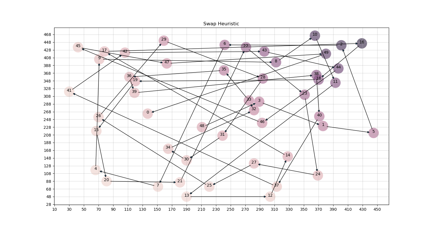
Swap Heuristic

Here, I explore the effect of repeatedly swapping the order in which a pair of adjacent cities are visited, as long as this swap improves (reduces) the cost of the overall tour. 

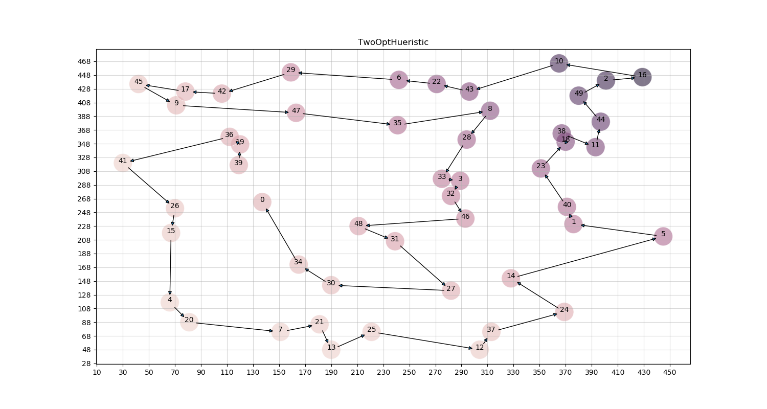
2-Opt Heuristic

The 2-Opt Heuristic is another heuristic that repeatedly makes local adjustments until there is no improvement from doing these. In this case, the alterations are more significant than the swaps.

This method repeatedly nominates a contiguous sequence of cities on the current tour and proposes that these be visited in the reverse order if that would reduce the overall cost of the tour.

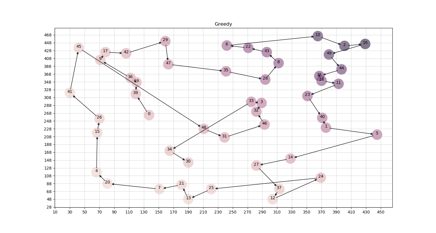
Greedy

A commonly used approach to optimization problems is the greedy approach, where at each step we do what seems best, and hope that this will lead to a globally optimal solution.

For the TSP problem, this approach involves taking some initial city/node (for us, we will take the one indexed 0) and building a tour out from that starting point. At the i-th step (for i= 0,…), we consider the recently-assigned endpoint in the path against all previously unused nodes, and then we take our next node to be the one closest in distance to the node at i. This will eventually create a permutation within the solution.

2-Approximation Algorithm

This is a bit sophisticated method, but requires the graph to follow the triangle inequality.

We start by computing an MST (minimum spanning tree) whose weight is a lower bound on the length of an optimal TSP tour. Then, use this MST to build a tour whose cost is no more than twice that of MST’s weight as long as the cost function satisfies the triangle inequality.

This website provides a better explanation and mathematics proof for more details http://www.personal.kent.edu/~rmuhamma/Algorithms/MyAlgorithms/AproxAlgor/TSP/tsp.htm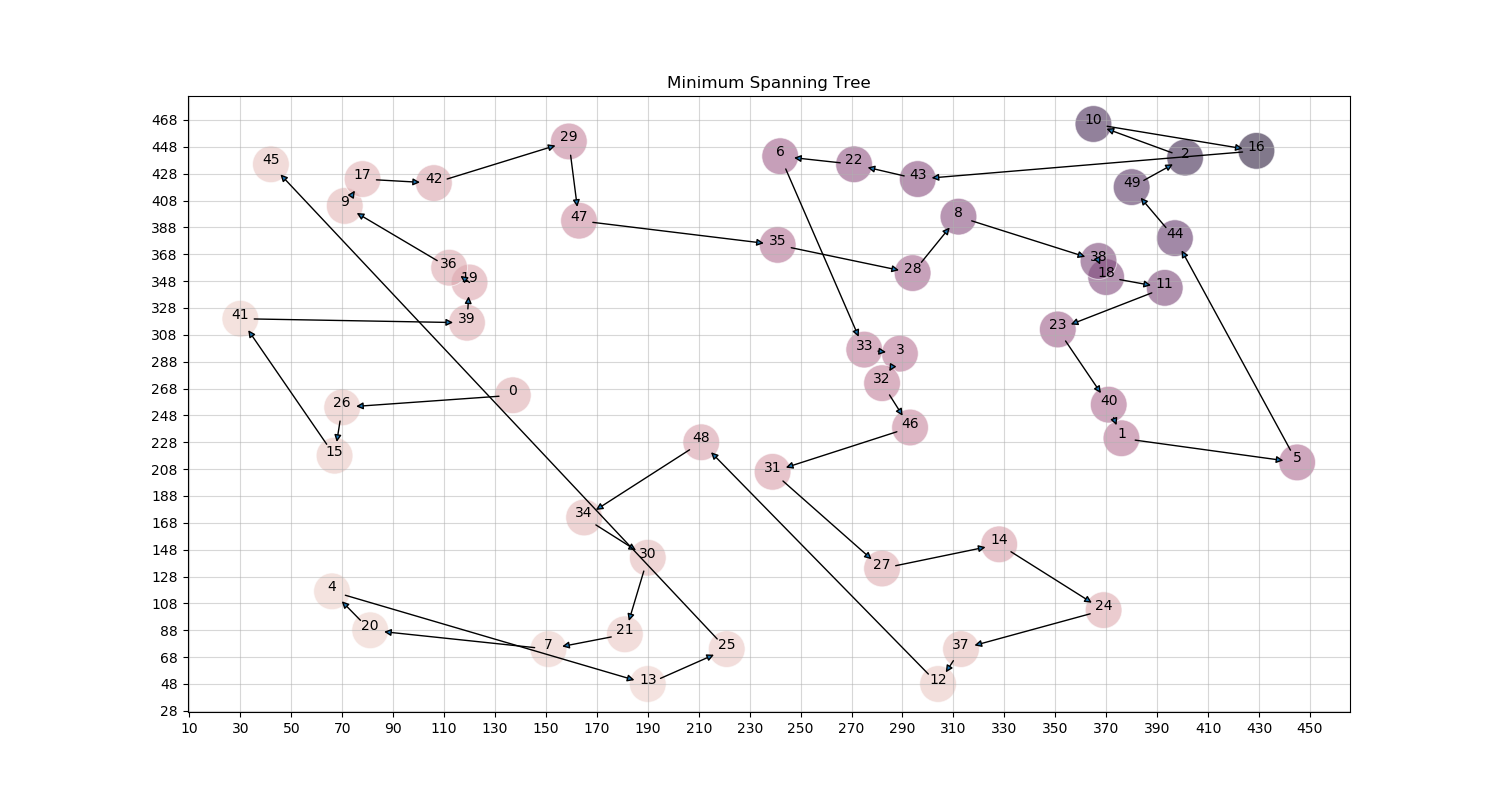 

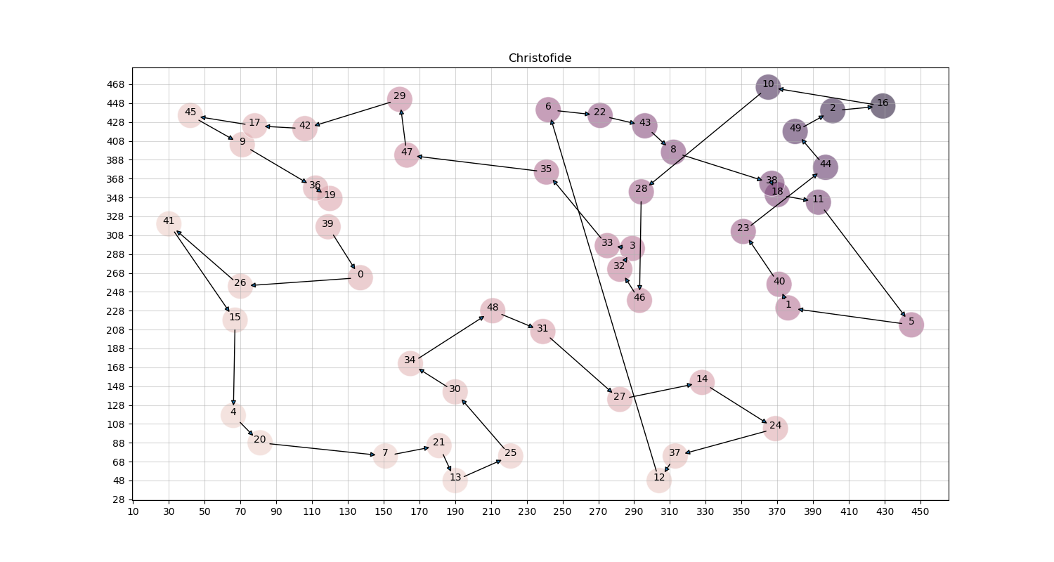
Christofides Algorithm

To tackle this, I did some research and found Christofide’s algorithm to be quite interesting which matched the above requirements. It claims to guarantee a solution within 1.5 errors.

Algorithm

It can be described in a few simple steps:

1. Find the minimum spanning tree T of the graph.
2. Find the Odd degree of vertices O. (They are even in number due to handshaking lemma.)
3. Find the minimum weight perfectly matching M from the vertices O.
4. Combine M and T to form an Eulerian circuit.
5. Now form a Hamiltonian circuit from the circuit in the previous step.

Proof for polynomial time.

The following are the running times for each of the above steps.

1. O(V2), I used Prim’s algorithm designed for the adjacency matrix. Note, that it can be improved to O(E.log(V) if using heaps.
2. O(V) Goes through all the vertices once.
3. O(V2). Note, that this does not find the perfect minimum weight matching. I decided to implement a greedy solution which gives an approximation of the perfect minimum weight matching.
4. O(V2). This just traverses the combined graph of M and T.
5. O(V). This removes any extra edges that occur.

As we can see, the algorithm consists of combining steps 1-5, and so it runs in O(V2) time, which is polynomial. I have annotated the algorithm in the implementation properly for you to verify it.

Proof for 1.5 error approximation

The weight of a minimum spanning tree is less than the optimal solution:

1. Take an optimal tour of cost OPT (optimal solution).
2. Drop an edge to obtain a tree T.
3. All distances are positive so cost(T) <= cost OPT, Hence cost(MST) <= cost OPT.

The two-approximation algorithm traverses the Minimum spanning tree twice, at most repeating all vertexes V, 2V times. Resulting in the cost to be doubled. Hence: $$ 𝑐𝑜𝑠𝑡(𝑀𝑆𝑇)<= 𝑂𝑃𝑇 <=2.𝑐𝑜𝑠𝑡(𝑀𝑆𝑇) $$ We improve this algorithm, by instead of traversing all the edge two times, we can make shortcuts between odd vertices. Therefore, the cost of the tour becomes: $$ 𝑐𝑜𝑠𝑡(𝑀𝑆𝑇)+𝑐𝑜𝑠𝑡(𝑃𝑒𝑟𝑓𝑒𝑐𝑡 𝑀𝑎𝑡𝑐ℎ𝑖𝑛𝑔 𝑃𝑀) $$

$$ 𝑐𝑜𝑠𝑡(𝑀𝑆𝑇)+𝑐𝑜𝑠𝑡(𝑃𝑀)≤𝑐𝑜𝑠𝑡(𝑂𝑃𝑇)+𝑐𝑜𝑠𝑡(𝑃𝑀) $$

Bounding, PM

1. Take an optimal tour of cost OPT.
2. Consider the odd vertices O.
3. Shortcut the path to only use O.
4. As they have perfect matchings, they partition into M1 and M2, such that cost(M1)+Cost(M2) <=OPT
5. Therefore Cost(PM) <=OPT/2.

$$ 𝑐𝑜𝑠𝑡(𝑀𝑆𝑇)+𝑐𝑜𝑠𝑡(𝑃𝑀)≤𝑐𝑜𝑠𝑡(𝑂𝑃𝑇)+𝑐𝑜𝑠𝑡(𝑂𝑃𝑇)/2 $$

Therefore, Christofide’s Algorithm is said to have a 1.5 approximation bound for TSP-metric problems.

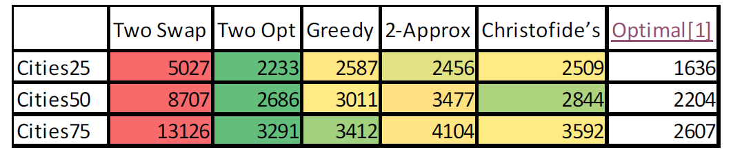
Testing

I have written the details for testing, in the test.py file followed by the high-level description in the pdf files.

Here is the overview: